![]()
Project ISC-MED-35 - EGOIST
Title:
Alternative Methods for the Optimization of Telecommunication
Networks
Author(s):
Olaf Barheine, Stefan Bergstedt, Alessandro Idili, and E. von
Goldammer
Organization(s):
Institut für Kybernetik & Systemtheorie - ICS
Keywords:
genetic algorithms, heuristic optimization, minimal spanning
trees, shortest paths algorithms
Address:
Institut für Kybernetik & Systemtheorie - ICS
Office: Harpener
Hellweg 532
D-44388 Dortmund
Tel & Fax (+49) 2302 - 80 20 16
email: ics@ics.prima.ruhr.de or vgo@xpertnet.de
Content:
Alternative Methods for the Optimization
of Telecommunication Networks
1 TELECOMMUNICATION NETWORKS AS A CONCEPT OF GRAPHS AND TREES
1.1.1 Structure of the Potential Network (P-NW)
1.1.2 Structure of the Optimized Network (O-NW)
1.2 Spanning Trees and Shortest Paths
1.2.1 Minimum Spanning Trees - MST
1.2.2 Shortest Paths: Dijkstra´s algorithm
1.2.3 Dynamic Costs: Limitations of MST and Shortest Paths Algorithms
2 THE APPROACH OF ICS WITHIN EGOIST
Alternative Methods for the Optimization of Telecommuncation Networks
In the context of the present project "alternative" optimization methods are all possible methods except genetic algorithms (GA). Since this classification is not very common, we will distinguish in the following between heuristic and non-heuristic, i.e., exact methods. The term heuristic derives from Greek ´heuriskein´, which means to find or discover. The word has been used in Artificial Intelligence circles with quite a different connotation - Pearl /1/, for example, uses the term to include methods such as branch-and-bound which find globally optimal solutions, and this usage probably pre-dates the now common one. In fact this usage is perfectly reasonable, if a heuristic is a "finding" method, one may ask what it is finding, if not a global optimum. What in Operational Research very often is called ´heuristic´ would be better described as a ´seeking´ method, as it cannot guarantee to find anything.
Thus in the following the term heuristic will be used as a contrast to methods which guarantee to find a global optimum. In other words, a heuristic method seeks good, i.e., near optimal, solutions at reasonable computational costs without being able to guarantee either feasibility or optimality, or even in many cases to state how close to optimality a particular feasible solution is.
As will be shown in the present survey, there is another strong argument in favor of heuristic methods. Since we are using models for optimizing a real- world problem, the question is, should we prefer an exact solution of an approximate model or an approximate solution of an exact model ?
Of course, one cannot hope for a truly exact model, but heuristics are usually rather more flexible and are capable of coping with more complicated (and more realistic) objective functions and/or constraints than exact algorithms.
This is the case for methods like genetic algorithms, mutation selection threshold algorithms, simulated annealing, etc. Within the present project mainly two heuristic methods have been used, namely genetic algorithms (GA) and mutation selection threshold algorithms (MSTA). A survey on these two methods and a variety of other heuristics was given in the ´three monthly report´ /2/ of the EGOIST project and will not be repeated in the present survey.
| 1. | Telecommunication Networks as a Concept of Graphs and Trees |
The idea of graphs is one of the most fruitful concepts in discrete mathematics. In fact there are many everyday problems which can be solved quite easily using the concept of graphs.
Some definitions (just for remembrance):
A graph is an ordered pair { V, E } in which V is a set called the vertex set (or set of nodes) and E is a set consisting of subsets of V with two elements. The set E is called the edge set, and a and b are called joined by an edge if { a, b} belongs to E.
A path is a sequence of vertices of a graph in which each successive pair of vertices is an edge of the graph.
A graph is connected if given any two distinct vertices there is a path from one to the other. A graph which is not connected is said to be disconnected.
A circuit is a path which starts and ends at the same vertex. A cycle is a circuit in which the initial vertex occurs twice and no other vertex is repeated.
A tree is a connected graph which has no cycles.
A spanning graph for G = { V, E } is a subgraph G´ = { V´, E´} such that V´= V.
A spanning tree for G is a spanning graph for G which is a tree.
| 1.1 | The Problem to be Solved |
The telecommunication network is given as a graph G with three types of nodes (or vertices). The network which has to be optimized contains all possible connections between the different nodes. Therefore this network will be called "the potential network: P-NW". In other words, the potential network is a graph which contains more nodes (vertices) and connections (edges) than the resulting network which will be called "the optimized network: O-NW". This has been shown in fig._1.
| 1.1.1 | Structure of the Potential Network (P-NW) |
The nodes can be classified as follows:
CCP: the central connection point of the network (vertex set: V1 );
UGR: underground room which is necessary for cable laying around edges
and/or cable branching or cable division ( vertex set: V2 );
DIP: distribution points (endpoints or leaves within the
telecommunication network) (vertex set: V3 ).
Fig._1: A potential network (P-NW) and the resulting optimized network
(O-NW)
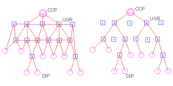
Potential Network : P-NW |
Optimized network : O-NW |
The P-NW is characterized by nodes (vertices) which are connected by undirected edges where the following rules hold:
- |
any DIP is connected with only one UGR; |
- |
in general the CCP is connected with only one UGR; |
- |
the DIPs cannot be connected directly with the CCP; |
- |
the paths of the graph are simple, i.e., no edge is repeated within a path; |
- |
there are no loops within the graph; |
- |
the DIPs are leaves within the graph; |
- |
the DIPs are weighted by their capacities. |
| 1.1.2 | Structure of the Optimized Network (O-NW) |
The network resulting from the optimization consists from paths starting from the DIPs to the CCP. A minimization of the costs results from an optimal compromise between a minimal length of the cable layout, a minimal number of UGRs and a minimal length of the total network, i.e., combining as many cable ropes as possible (cf. fig. 2). Thus the resulting O-NW does not contain cycles which are also meaningless in a telecommunication network from a physical point of view. The resulting O-NW is a connected graph without cycles, i.e., it is a tree with the CCP as root and the DIPs as leaves. As it can be seen from fig._1 and fig._2 the set of UGRs (set of vertices V´2 ) in the resulting network is smaller than the corresponding set in the potential network, viz.,
| P-NW is a graph | |
| O-NW is a graph | |
with |
The set of vertices/nodes (UGRs) V´2 and edges/connections E´ within the O-NW are subsets of V2 and E, the sets of the UGRs and connections within the potential network, P-NW.
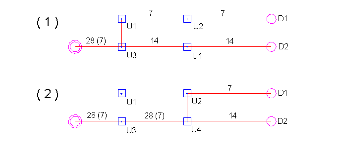
For demonstration purposes Fig._2 reveals two possible configurations of a cable layout with different numbers of UGRs resulting from varying combinations of the cable capacities, i.e., the combined number of cable ropes.
Fig._2: Varying cable layout resulting in different numbers of UGRs.
( 1 ): UGRs necessary: U1, U3 and ( 2 ): UGRs necessary: U4
- the number in brackets reflect the free capacity of the corresponding cable.
| 1.2 | Spanning Trees and Shortest Paths |
As long as the cabling costs are fixed (static - see below) as shown, for example, in fig._2 then any algorithm which transforms a graph into a tree can be considered as a possible candidate for optimizing the P-NW. Since every connected graph has at least one spanning tree, the simplest approach is to find this spanning tree, viz.,
ALGORITHM_SPAN
{ Takes a connected graph and finds a spanning tree}
begin
while cycles exist in G do
remove an edge form a cycle of G
od
end
Since this algorithm is extremely simple it can be executed just for demonstration purposes as a ´paper and pencil´ example. Fig._3 shows a graph with three classes of nodes as it occurs for the potential telecommunication networks and two resulting spanning trees.
Fig._3: Construction of spanning trees
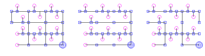
graph |
spanning tree_1 |
spanning tree_2 |
| 1.2.1 | Minimum Spanning Trees - MST |
As it can be seen in fig._3, it is possible to cancel some of the UGRs within the spanning trees_1 and _2 (e.g., UGRs as leaves and/or UGRs in a path without an angular displacement are meaningless). In other words, this example demonstrates that a reduction of UGRs and the cable length occurs if a spanning tree has been constructed. Thus introducing the idea of weighted graphs (cost functions) gives an opportunity to optimize a telecommunication network in the sense of an exact algorithm - provided the costs are not varying with the configuration of the resulting network structure. If this is the case we are speaking of dynamic costs, which will be discussed below.
A tree of minimum total cost is called a minimum spanning tree. Several algorithms for finding minimal spanning trees are known and discussed in the literature (a good survey is given in ref./3/). Here only Kruskal´s and Prim´s algorithm should be mentioned. For more details see ref.3.
| 1.2.2 | Shortest Paths: Dijkstra´s algorithm |
So far as the role of the DIP´ s and the CCP is concerned the potential network already has a pre-defined structure, i.e., the DIPs are always the leaves and the CCP is the root in the resulting spanning tree. In other words, the optimization belongs to the problems of finding the shortest paths in a directed and weighted graph between a given initial node (CCP as a root of the final tree) and the DIPs (as leaves in the final tree).
Dijkstra´s algorithm keeps track of two sets of vertices/nodes. The set S consists of all vertices to which a shortest path from the given initial vertex has to be found. The set T consists of all the rest of the vertices. When the algorithm begins, S consists of only the initial vertex, and with each iteration of the algorithm, a vertex is removed from T and placed in S. When the desired final vertex is placed in S, the process stops. The algorithm keeps track of the path used to reach each vertex and maintains data on the shortest actual distance (for vertices in S) as well as an estimate of the shortest distance to each vertex in T.
The estimates of the distances for each vertex in T are based on paths which include only vertices in S, expect for the last vertex. It can be shown that the shortest estimated distance to any vertex in T is indeed correct, so that the vertex in T with the shortest estimated distance will be the one added to S (and removed from T). Once the new vertex is added to S, the estimated distances to the vertices remaining in T are updated and the process is repeated.
Fig._4: Shortest path from A
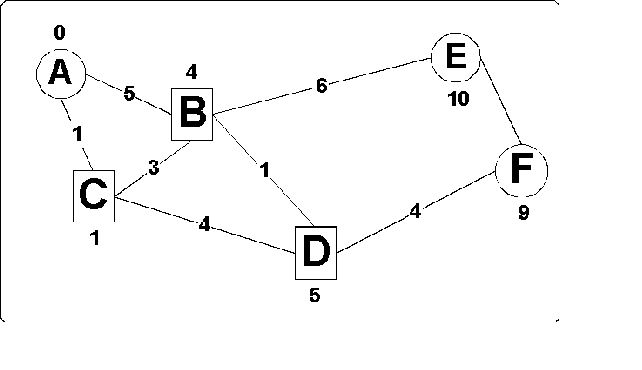
As an example, consider the network shown in fig._4. The objective is to find the shortest paths, i.e. the paths with minimum costs /4/, form A to all other vertices/nodes. Initially the set S = { A} , and thus T = { B, C, D, E, F} . The distance to A is known (it is zero), and its label is 0 and all other nodes have labels of infinity. Scanning node A -> B is assigned a label of 5 and A -> C a label of 1. The shortest estimated distance is the one to C. We thus remove C from set T and place it to S. We also retain the information that the paths to each of B and C end with an edge from A.
The next step is to revise the estimated
distances (costs) for the nodes still remaining in T.
The estimates are based on using paths remaining in S
except for the final edge. To determine whether a better path
could be found which passes through the vertex C
that was just added to S. Since
the distance to A was 1, we simply add 1
to the distance from A to B,
D, E, and F.
If this result is smaller, then the new best path to that vertex
would be to go to A and to follow the
edge from A to that vertex. This does
cause us to change the estimated distance to the vertex B
to a value of 4 (=1+3; now the path to B
is by way C). We now find that the vertex
in T with the smallest estimate
distance is B, with a distance of 4. We
remove D from T
and put it in S.
At this point S = { A, C, B}
, and T = { D, F, E}
.
The process continues as we revise the estimated distances (costs) again. Now the estimate gives the distance for D of 5 (4+1) and for E of 10 (4+6). The process continues with D going to the set S, a revised value of 9 being calculated for F, and finally F being placed to S. At the same time we retained the fact that (after revisions) the last vertex preceding F was D and preceding D was B. Since B was preceded by C and C by A, the final path is ACBDE with a length of 9 and ACBE with a length of 10, if E and F are considered as leaves (DIPs) in the resulting tree.
Each node has been scanned at most once. Note that all edges in the paths from A to all other nodes, i.e., { A,C} , { C,B} , { B,D} , { B,E} , and { D,F} form a tree. This is not a coincidence but a direct consequence of the fact that the shortest paths nest within one another. For example, if k is on the shortest path form i to j then the shortest path form i to j include the shortest path from i to k and the shortest path from k to j. All shortest path algorithm rely on the observation, that shortest paths nest.
Dijkstra´s algorithm can be used with weighted undirected graphs as well as with directed graphs. Besides Dijkstra there are several other shortest paths algorithms such as Bellman´s or Floyd´s algorithm (for more details cf. ref.3).
| 1.2.3 | Dynamic Costs: Limitations of MST and Shortest Paths Algorithms |
If the total number of the underground rooms (UGRs) together with the total length of the cable within a network and/or the length between the nodes would have to be considered as the determining cost factors, then the optimization could be done by one of the shortest paths algorithms. However, as it was already mentioned above, there are so-called dynamic costs which depend strongly on the structure of the resulting (optimized) network.
Fig._5: Dynamic costs
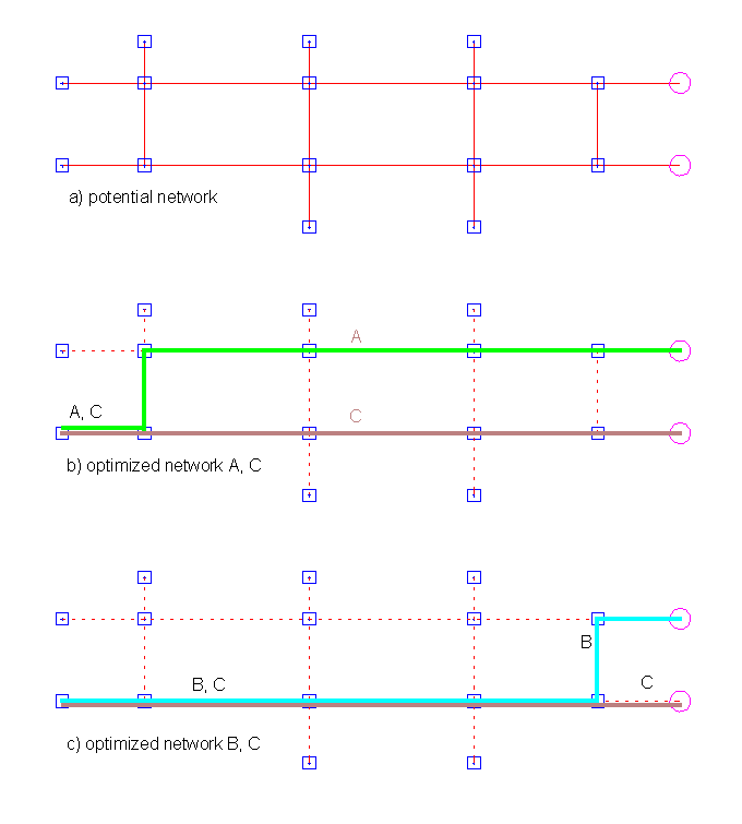
Although the constraints will be collected not before the next chapter, an example will be given in order to demonstrate the shortcomings of the MST and the shortest paths algorithms for an efficient optimization of the problem within EGOIST project.
Fig._5 shows three different paths labeled as A, B, and C. If the costs depend only on the length and/or the number of UGRs, then the costs of the paths (A+C) would be the same as for (B+C). As it was shown in fig._2, cables can be combined, i.e., cables with a higher number of wires are less expensive. In case of the example in fig._5 this means that the costs of (A+C) are less than for (B+C), viz.,
Static Constraints/Costs:
length_of_path [ A + C] = length_of_path [ B + C]
fixed_costs [ A + C] = fixed_costs [ B + C]
Dynamic Constraints/Costs
dynamic_costs [ A + C] < dynamic_costs [ B + C]
In order to consider the dynamic constraints (costs) which strongly depend on the specific structure of the resulting tree, heuristic methods are rather more flexible than the exact algorithm which is hard to find for the present optimization task.
| 1.3 | Constraints |
In the following list, the constraints have been collected using a terminology as if the cable laying will be performed from the DIPs to the CCP. It is important to note that in reality the cable laying will be performed from the CCP to the DIPs. It is simply a matter of semantics if we are speaking from combining instead of dividing cables as it will be done below if we are looking from the DIPs to the CCP.
The following constraints only consider local networks in a smaller city area (with only one connection point, CCP). For larger networks, for example, for a whole city similar constraints have to be considered. For these cases, however, the cable capacities, the number of CCPs, etc. will be different.
| 1) | Size of the cable (number
of wires within a cable rope): N=7× 2n with n as an integer in the range 0 Ł n Ł 6 (N = 7, 14, 18, 56, Ľ , 448). |
| 2) | Diameter (Q) of the cable: Q = { 0.4mm2, 0.6mm2, 0.8mm2 } The decision about the diameter is done in advance depending on the total laying length and the total electrical resistance. |
| 3) | Combining of cable ropes:
|
| 4) | Parallel laying of cable
ropes within one connection: Parallel laying is only allowed if combining of the ropes is not possible. |
| 5) | Cable branching: If there is a cable with a capacity of N and an unused capacity of N/4 it is possible to connect a cable with N/4 - the resulting capacity again is N. |
| 6) | Maximum length of cables: For the local networks the given maximum length of ...m is to high in order to be installed. |
| 7) | Necessity for the
installation of an UGR: For the combining of cables; If only a DIP has to be connected a UGR is not necessary. Angular variations (more than 100) for cable laying. |
| 8) | Types of UGRs The type depends on highest value N of the cable capacity and the diameter Q of the cables. |
| 9) | DIP capacity It is given as N = 7× 2n (see above) |
| 10) | Types of tubes For the laying of the cables tubes are used. The type (size) of the tubes depends on the capacity and the diameter of the cables. |
| 11) | Laying of the cable The laying of the cables is done in tubes, the kind of laying depends on the combination of the number of type of tubes. |
| 1.4 | Costs |
Since the costs are strongly case dependent, i.e., they differ, for example, from one country to another, a data base application was written in order to make the optimization tool independent from the conditions in Tunisia.
| 1) | Cables (see, DB-table:
cable.dbf)
|
| 2) | Laying of cables (see,
DB-table: laying.dbf):
|
| 3) | Installation of UGR (see,
DB-table: ugr.dbf):
|
| 4) | Combining of cables (see,
DB-table: cable.dbf):
|
Data base files:
cable.dbf
CAPACITY |
CALIBER |
CABLECOSTS |
DIVCOSTS |
TUBETYPE |
7 |
0.4 |
0.44 |
0 |
1 |
7 |
0.6 |
0.44 |
0 |
1 |
7 |
0.8 |
0.44 |
0 |
1 |
14 |
0.4 |
0.577 |
10 |
1 |
14 |
0.6 |
0.577 |
10 |
1 |
14 |
0.8 |
0.577 |
10 |
1 |
28 |
0.4 |
0.844 |
15 |
1 |
28 |
0.6 |
0.844 |
15 |
1 |
28 |
0.8 |
0.844 |
15 |
1 |
56 |
0.4 |
1.5 |
18 |
1 |
56 |
0.6 |
1.5 |
18 |
1 |
56 |
0.8 |
1.5 |
18 |
1 |
112 |
0.4 |
2.7 |
23 |
1 |
112 |
0.6 |
2.7 |
23 |
1 |
112 |
0.8 |
2.7 |
23 |
2 |
224 |
0.4 |
5 |
27 |
1 |
224 |
0.6 |
5 |
27 |
1 |
224 |
0.8 |
5 |
27 |
2 |
448 |
0.4 |
9.9 |
40 |
1 |
448 |
0.6 |
9.9 |
40 |
2 |
448 |
0.8 |
9.9 |
40 |
3 |
laying.dbf:
TUBE_3 |
TUBE_2 |
TUBE_1 |
CABLE_3 |
CABLE_2 |
CABLE_1 |
COSTS |
0 |
0 |
2 |
0 |
0 |
1 |
6.5 |
0 |
0 |
3 |
0 |
0 |
1 |
7.3 |
0 |
0 |
4 |
0 |
0 |
2 |
8 |
0 |
0 |
5 |
0 |
0 |
3 |
8.8 |
0 |
0 |
6 |
0 |
0 |
4 |
9.6 |
0 |
2 |
0 |
0 |
1 |
0 |
7.5 |
0 |
2 |
2 |
0 |
1 |
1 |
9 |
0 |
3 |
2 |
0 |
1 |
1 |
10.2 |
0 |
4 |
3 |
0 |
2 |
1 |
13.1 |
ugr.dbf:
TYP |
MAX0_4 |
MAX0_6 |
MAX0_8 |
LENGTH |
WIDTH |
HIGH |
COSTS |
A2 |
112 |
112 |
56 |
1.13 |
0.77 |
0.835 |
166 |
A3 |
1.45 |
0.77 |
0.835 |
||||
A4 |
224 |
224 |
112 |
2.1 |
0.77 |
0.835 |
155 |
B2 |
448 |
448 |
224 |
2.9 |
1.29 |
1.58 |
170 |
B3 |
3.5 |
1.29 |
1.58 |
||||
C2 |
4 |
1.8 |
2.64 |
1395 |
|||
D1 |
2.34 |
1.25 |
1.91 |
||||
D2 |
2.34 |
1.25 |
1.91 |
917 |
|||
D3 |
3.7 |
1.75 |
2.68 |
||||
D4 |
4.2 |
2 |
2.68 |
tube.dbf:
TUBETYPE |
DIAM_I |
DIAM_O |
1 |
42 |
45 |
2 |
56 |
60 |
3 |
75 |
80 |
| 1.5 | Résumé |
There are many treatments of graphs in order to find minimum spanning trees or shortest paths. All algorithms for calculating minimum spanning trees are not suitable for the present optimization problem where the graphs already are pre-defined with DIPs as leaves and the CCP as a root.
The Dijkstra algorithm and all the other shortest paths algorithms are very well suited for a search of an optimal tree as long as the cost functions do not depend on the resulting structure. In other words the Dijkstra algorithm gives good results for the optimization of a network (graph) with fixed (or better with static) costs. For cases where the cost function depends on the structure of the resulting network, the calculations have to be done in two steps. Shortest paths algorithms are looking for all shortest paths between the CCP and the DIPs. Since there might be several possible paths with (nearly) identical (static) costs, the algorithm selects only one of these paths as an optimal solution. However, considering the variable, i.e., the dynamic costs, such a selection might not be an optimal one. In order to change this within the shortest paths algorithms one has to develop a complete new formulation, i.e., a new algorithm. At the moment an exact algorithm does not exist for the optimization of networks with static and dynamic costs.
The following example has been given in order to demonstrate the principal difficulties in solving an optimization problem with dynamic costs.
example limitations of shortest_paths_algorithms
for the EGOIST problem:
The result of shortest_path_algorithms (e.g., Dijkstra) are paths from the DIPs to the CCP with minimum (static) costs (the "shortest" path is a path between a DIP and the CCP with minimum static costs):
path_1 DIP1 - CCP
path_2 DIP2 - CCP
path_3 DIP3 - CCP
path_4 DIP4 - CCP
etc. etc.
An optimization concerning the dynamic costs will be obtained by combining paths (or parts of paths) where the conditions for a combining are given.
Example:
There is a path_2´ that was not calculated by the shortest_path_algorithm because its static costs are (slightly) higher than those of path_2, i.e.,
static_costs[ path_2] < static_costs[ path_2´]
With path_2´, however, it could be possible to combine a larger part of cables, for example, with path_1. So as a result the dynamic costs of the combination of path_1 and path_2´ are lower than costs for the combination of path_1 and path_2, i.e.,
costs[ comb(path_1,path_2´)] < costs[ comb(path_1,path_2)]
It is obious that such a situation cannot be considered by means of any exact algorithm, especially if both combined paths do not belong to the class of minimum shortest paths, such as, for example, path_1´and path_2´, so that
costs[ comb(path_1´,path_2´] < costs[ comb(path_1,path_2´)]
Both path_1´ and path_2´ would not result from a shortest_path_algortihm - this is the problem.
| 2. | THE APPROACH OF ICS WITHIN EGOIST |
Within the EGOIST project three different optimization tools have been developed by the ICS:
EGONET
This is a tool based on a Genetic Algorithm which is written in ANSI-C, i.e., the tool can be implemented on all platforms. EGONET was tested under Unix/Linux, OS/2, Windows 3.11 and Windows 95.
Mutation_Selection-Threshold_Accepting (MS-TA)
This tool also is written in ANSI-C and therefore can be implemented on different operating systems.
Dijkstra´s algoritm
At the beginning of EGOIST some experiments have been done with Krkuskal´s and Prim´s algorithm for the calculation of minimum spanning trees. It turned out, however, that the search for minimum spanning trees is not very suitable for graphs with a per-defined root and leaves. Therefore Dijkstra´s algorithm was tested which produced good results as long as the cost function was considered as a static function. Later in the project it turned out that dynamic costs are extremely important and this was the end of the experiments with shortest paths algorithms such as Dijkstra´s algorithm.
CAD-functions
Since the optimization has to be performed on manually drawn (analogue) maps, the tool was implemented into a CAD software package. For this implementation the data exchange format is of great importance. Therefore a standard (vector) format was defined at the beginning of the project. The CAD functions of the tool are necessary for the construction of the potential telecommunication network (P-NW). This (computer aided) construction can done with the developed tool by using the corresponding bitmap as background. The bitmap can be obtained simply by scanning the manually drawn (paper) map. At the moment, however, the CAD software is in German but the optimization tools can be implemented into other CAD systems.
Data base application
Since the costs are variable, i.e., they may differ for applications in other countries (e.g., in Tunisia no manpower costs for digging was considered) a data base application (dBase III) was developed and implemented to the CAD software package. Again ANSI standards have been used in order to have a platform independent product.
The developed solution can be represented as it is shown in fig._6:
Fig._6: The tool developed by ICS
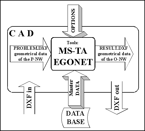
Details on the optimization tools MS-TA and EGONET have been reported periodically within the monthly and quarterly reports. They will be summarized within the final report at the end of the EGOIST project.
For the networks analyzed so far there was no difference in the performance of both tools.
The tools also can be used with some minor modifications for the optimization of utility networks.
| 1 | Pearl, J., Heuristics,
Addison-Wesley, Reading, Mass., 1984 |
| 2 | Optimization: Methods and
Tools (O. Barheine, S. Bergstedt, A. Idili, and
E.v.Goldammer, eds.), Project ISC-MED-35-EGOIST, 1995 |
| 3 | Kershenbaum, A.,
Telecommunication Network Design Algorithms, McGraw Hill
Publ., N.Y., 1993 |
| 4 | In the present context the
meaning of "shortest path" is "minimum
(static) costs" |
| 5 | Note that specific
manpower costs (e.g., for digging etc.) are not
considered in Tunisia. In other countries the manpower
costs for digging depend on so-called soil classes.In
order to consider these cases for other applications, a
data base has been implemented. |
![]()
webmaster@xpertnet.de
Copyright ©: 1996, ICS
last revised Jan. '97